5. Performing analyses
ivy has many tools for performing analyses on trees. Here we will cover
a few analyses you can perform.
5.1. Phylogenetically Independent Contrasts
You can perform PICs using ivy‘s PIC function. This function takes a
root node and a dictionary mapping node labels to character traits as inputs
and outputs a dictionary mappinginternal nodes to tuples containing ancestral
state, its variance (error), the contrast, and the contrasts’s variance.
The following example uses a consensus tree from Sarkinen et al. 2013 and Ziegler et al. unpub. data.
Note: This function requires that the root node have a length that is not none. Note: this function currently cannot handle polytomies.
In [1]: import ivy
In [2]: import csv
In [3]: import matplotlib.pyplot as plt
In [4]: r = ivy.tree.read("examples/solanaceae_sarkinen2013.newick")
In [5]: r.length = 0
In [6]: polvol = {}; stylen = {}
In [7]: with open("examples/pollenvolume_stylelength.csv", "r") as csvfile:
            traits = csv.DictReader(csvfile, delimiter = ",", quotechar = '"')
            for i in traits:
                polvol[i["Binomial"]] = float(i["PollenVolume"])
                stylen[i["Binomial"]] = float(i["StyleLength"])

In [8]: p = ivy.contrasts.PIC(r, polvol) # Contrasts for log-transformed pollen volume
In [9]: s = ivy.contrasts.PIC(r, stylen) # Contrasts for log-transformed style length
In [10]: pcons, scons = zip(*[ [p[key][2], s[key][2]] for key in p.keys() ])
In [11]: plt.scatter(scons,pcons)
In [12]: plt.show()
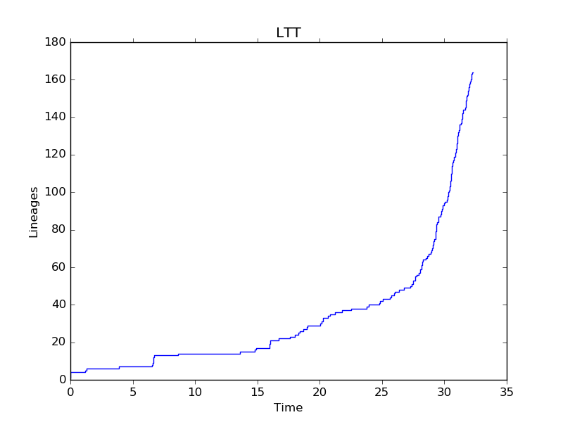
5.2. Lineages Through Time
ivy has functions for computing LTTs. The ltt function takes a root
node as input and returns a tuple of 1D-arrays containing the results of
times and diverisities.
Note: The tree is expected to be an ultrametric chromogram (extant leaves, branch lengths proportional to time).
In [13]: import ivy
In [14]: r = ivy.tree.read("examples/solanaceae_sarkinen2013.newick")
In [15]: v = ivy.ltt(r)
You can plot your results using matplotlib.
In [16]: import matplotlib.pyplot as plt
In [17]: plt.step(v[0], v[1])
In [18]: plt.xlabel("Time"); plt.ylabel("Lineages"); plt.title("LTT")
In [19]: plt.show()

5.3. Phylorate plot
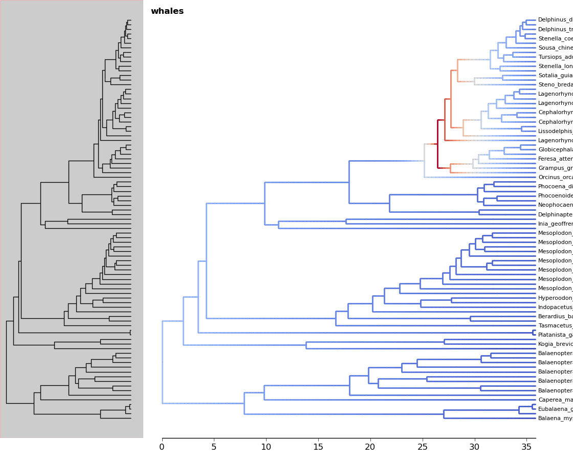
By accessing R libraries using rpy2, we can use the functions in the BAMMtools R library to generate phylorate plots.
The following analysis is done using the whales dataset provided with BAMMtools.
In [20]: from ivy.r_funcs import phylorate
In [21]: e = "whaleEvents.csv" # Event data created with BAMM
In [22]: treefile = "whales.tre"
In [23]: rates = phylorate(e, treefile, "netdiv")
We can add the results as a layer to a plot using the add_phylorate function
in ivy.vis.layers
In [24]: from ivy.vis import layers
In [25]: r = readtree(treefile)
In [26]: fig = treefig(r)
In [27]: fig.add_layer(layers.add_phylorate, rates[0], rates[1], ov=False,
       store="netdiv")

5.4. Mk models
ivy has functions to fit an Mk model given a tree and a list of character
states. There are functions to fit the Mk model using both maximum likelihood
and Bayesian MCMC methods.
To fit an Mk model, you need a tree and a list of character states. This list should only contain integers 0,1,2,...,N, with each integer corresponding to a state. The list of characters should be provided in preorder sequence.
Let’s read in some example data: plant habit in tobacco. We can load in a
csv containing binomials and character states using the loadChars function.
This gives us a dictionary mapping binomials to character states.
In [28]: tree = ivy.tree.read("examples/nicotiana.newick")
In [29]: chars = ivy.tree.load_chars("examples/nicotianaHabit.csv")
Let’s get our data into the correct format: we need to convert chars into a list of 0’s and 1’s matching the character states in preorder sequence
In [30]: charsPreorder = [ chars[n.label]["Habit"] for n in tree.leaves() ]
In [31]: charList = map(lambda x: 0 if x=="Herb" else 1, charsPreorder)
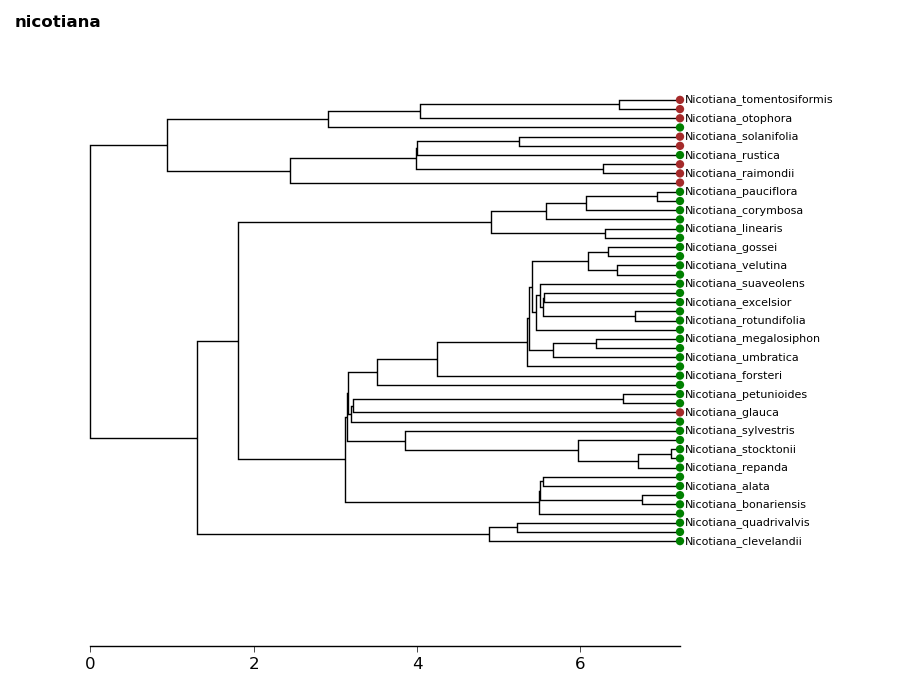
We can take a look at how the states are distributed on the tree using the
tip_chars method on a tree figure object. In this case “Herb” will be
represented by green and “Shrub” will be represented by brown.
In [32]: fig = ivy.vis.treevis.TreeFigure(tree)
In [33]: fig.tip_chars(charList, colors=["green", "brown"])

Now we are ready to fit the model. We will go over the maximum likelihood approach first.
5.4.1. Maximum Likelihood
Perhaps the simplest way to fit an Mk model is with the maximum likelihood
approach. We will make use of the optimize module of scipy to find
the maximum likelihood values of this model.
First, we must consider what type of model to fit. ivy allows you to specify what kind of instantaneous rate matrix (Q matrix) to use. The options are:
- “ER”: An equal-rates Q matrix has only one parameter: the forward and backswards rates for all characters are all equal.
- “Sym”: A symmetrical rates Q matrix forces forward and reverse rates to be equal, but allows rates for different characters to differ. It has a number of parameters equal to (N^2 - N)/2, where N is the number of character states.
- “ARD”: An all-rates different Q matrix allows all rates to vary freely. It has a number of parameters equal to (N^2 - N).
In this case, we will fit an ARD Q matrix.
We also need to specify how the prior at the root is handled. There are a few ways to handle weighting the likelihood at the root:
- “Equal”: When the likelihood at the root is set to equal, no weighting is given to the root being in any particular state. All likelihoods for all states are given equal weighting
- “Equilibrium”: This setting causes the likelihoods at the root to be weighted by the stationary distribution of the Q matrix, as is described in Maddison et al 2007.
- “Fitzjohn”: This setting causes the likelihoods at the root to be weighted by how well each root state would explain the data at the tips, as is described in Fitzjohn 2009.
In this case we will use the “Fitzjohn” method.
We can use the fitMk method with these settings to fit the model. This
function returns a dict containing the fitted Q matrix, the log-likelihood,
and the weighting at the root node.
In [34]: from ivy.chars import mk
In [35]: mk_results = mk.fit_Mk(tree, charList, Q="ARD", pi="Fitzjohn")
In [36]: print mk_results["Q"]
[[-0.01246449  0.01246449]
 [ 0.09898439 -0.09898439]]
In [37]: print mk_results["Log-likelihood"]
-11.3009106093
In [38]: print mk_results["pi"]
{0: 0.088591248260230959, 1: 0.9114087517397691}
Let’s take a look at the results
In [39]: print mk_results["Q"]
[[-0.01246449  0.01246449]
 [ 0.09898439 -0.09898439]]
First is the Q matrix. The fitted Q matrix shows the transition rate from i->j, where i is the row and j is the column. Recall that in this dataset, character 0 corresponds to herbacious and 1 to woody. We can see that the transition rate from woody to herbacious is higher than the transition from herbacious to woody.
In [40]: print mk_results["Log-likelihood"]
-11.3009106093
Next is the log-likelihood. This is the log-likelihood of the data using the fitted model
In [41]: print mk_results["pi"]
{0: 0.088591248260230959, 1: 0.9114087517397691}
Finally we have pi, the weighting at the root. We can see that there is higher weighting for the root being in state 1 (woody).
5.4.2. Bayesian
ivy has a framework in place for using pymc to sample from a Bayesian
Mk model. The process of fitting a Bayesian Mk model is very similar to fitting
a maximum likelihood model.
The module bayesian_models has a function create_mk_model that takes
the same input as fitMk and creates a pymc model that can be sampled
with an MCMC chain
First we create the model.
In [42]: from ivy.chars import bayesian_models
In [43]: from ivy.chars.bayesian_models import create_mk_model
In [44]: mk_mod = create_mk_model(tree, charList, Qtype="ARD", pi="Fitzjohn")
Now that we have the model, we can use pymc syntax to set up an MCMC chain.
In [45]: import pymc
In [46]: mk_mcmc = pymc.MCMC(mk_mod)
In [47]: mk_mcmc.sample(4000, burn=200, thin = 2)
[-----------------100%-----------------] 2000 of 2000 complete in 4.7 sec
We can access the results using the trace method of the mcmc object and
giving it the name of the parameter we want. In this case, we want “Qparams”
In [48]: mk_mcmc.trace("Qparams")[:]
array([[ 0.01756608,  0.07222648],
   [ 0.03266443,  0.05712813],
   [ 0.03266443,  0.05712813],
   ...,
   [ 0.01170189,  0.03909211],
   [ 0.01170189,  0.03909211],
   [ 0.00989616,  0.03305975]])
Each element of the trace is an array containing the two fitted Q parameters. Let’s get the 5%, 50%, and 95% percentiles for both parameters
In [49]: import numpy as np
In [50]: Q01 = [ i[0] for i in mk_mcmc.trace("Qparams")[:] ]
In [51]: Q10 = [ i[1] for i in mk_mcmc.trace("Qparams")[:] ]
In [52]: np.percentile(Q01, [5,50,95])
Out[52]: array([ 0.00308076,  0.01844342,  0.06290078])
In [53]: np.percentile(Q10, [5,50,95])
Out[53]: array([ 0.03294584,  0.09525662,  0.21803742])
Unsurprisingly, the results are similar to the ones we got from the maximum likelihood analysis
5.6. BAMM-like Mk model
ivy has code for fitting a BAMM-like
Mk model (also referred to here as a multi-mk model) to a tree, where different
sections of the tree have distinct Mk models associated with them.
We will demonstrate fitting a two-regime BAMM-like Mk model in a Bayesian context using pymc
In [66]: import ivy
In [67]: from ivy.chars import mk_mr
In [68]: from ivy import examples
In [69]: tree = examples.simtree_600
In [70]: chars = examples.simchar_600

In [71]: data = dict(zip([n.label for n in tree.leaves()],chars))
First, we will use the ivy function mk_multi_bayes to create the pymc
obejct. We will specify the model using a special array, the qidx array. The
qidx array provides information for fitting parameters into a Q matrix.
The qidx for a multi-mk model is a two-dimensional numpy array with four
columns. The first column refers to regime, the second column refers to the row index
of the Q matrix, and the third column refers to the column index of the Q matrix.
The fourth row refers to the parameter identity that will be filled into this
location.
TODO: link to mk_multi_bayes documentation
In this case, we will fit a model where there are two equal-rates mk models
somewhere on the tree, each with two different rates. The qidx will be
as follows:
In [72]: import numpy as np
In [73]: qidx = np.array([[0,0,1,0],
                         [0,1,0,0],
                         [1,0,1,1],
                         [1,1,0,1]])
In [74]: my_model = mk_mr.mk_multi_bayes(tree, data,nregime=2,qidx=qidx)
Now we will sample from our model. We will do 100,000 samples with a burn-in of 10,000 and a thinning factor of 3.
In [75] my_model.sample(100000,burn=10000,thin=3)
Now we can look at the output. Seeing the fitted parameters is easy.
In [76]: print(np.mean(my_model.trace("Qparam_0")[:])) # Q param 0
In [77]: print(np.mean(my_model.trace("Qparam_1")[:])) # Q param 1
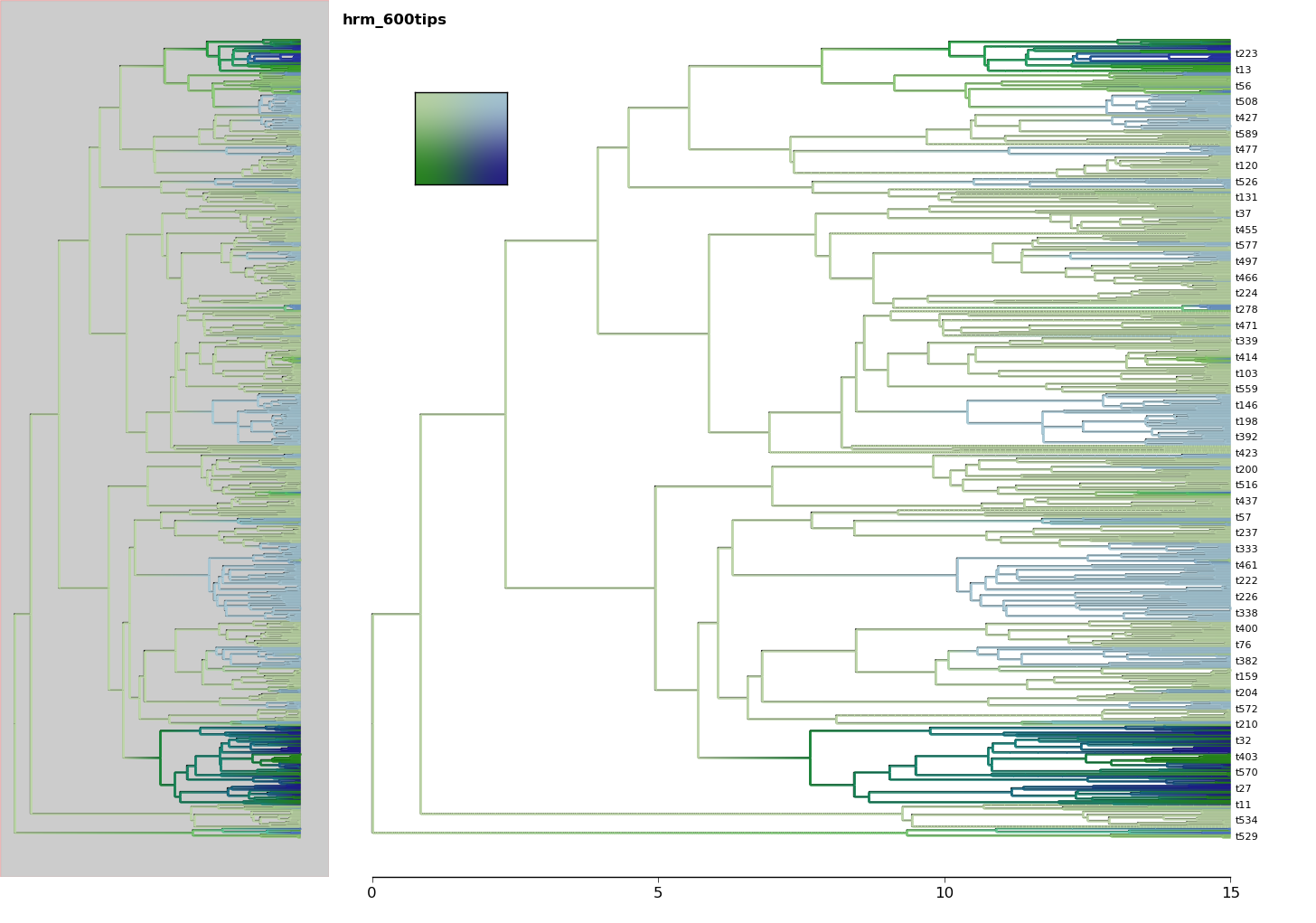
Seeing the location of the fitted switchpoints is a little trickier. We can
use the plotting layer add_tree_heatmap to see where the switchpoint
was reconstructed at.
In [78]: from ivy.interactive import *
In [79]: fig = treefig(tree)
In [80]: switchpoint = my_model.trace("switch_0")[:]
In [81]: fig.add_layer(ivy.vis.layers.add_tree_heatmap,switchpoint)

5.7. Classe
The ClaSSE model is implemented in ivy. Using ivy‘s ClaSSE implementation,
you can fit ClaSSE, along with all of its derivatives like GeoSSE, to your data.
When you fit a ClaSSE model, you get an output dictionary containing the log-likelihood and all fitted parameters.
The output is a dictionary containing the maximum log-likelihood and a dictionary containing the parameters.
The structure of the parameter dictionary is as follows: the dictionary contains three arrays; “lambda”, “mu”, and “q”.
The lambda array is a three-dimensional array that corresponds to the speciation rates. The first dimension corresponds to the parent’s state, the second to the first child’s state, and the third to the second child’s state. Thus, lambda[0,0,1] corresponds to the speciation rate where the parent is in state 0, the first child is in state 0, and the second child is in state 1. As in diversitree, any lambda values where the first child has a higher state than the second child (e.g. lambda[0,1,0]) is set to 0.
The q array is a two-dimensional array that corresponds to the rates of character change. The first dimension corresponds to the rootward state and the second dimension corresponds to the tipward state. q[0,1] corresponds to the transition rate from 0 to 1. The diagonals are set to zero.
The mu array is a one-dimensional array. It corresponds to the extinction rate of each state. mu[0] corresponds to the extinction rate of state 0.
We will demonstrate fitting a fully-parameterized 2-state ClaSSE model to some data, then fitting a 3-state ClaSSE model that has been parameterized to be identical to GeoSSE.
In [82]: import ivy
In [83]: from ivy.chars.sse import sse
In [84]: from ivy import examples
In [85]: root = examples.simtree_600 # This is an ivy Node object
In [86]: data = examples.simdata_600 # This is a dictionary mapping tip labels to character states
5.7.1. Maximum likelihood ClaSSE
Fitting a model is relatively straightforward with fit_classe.
This implementation is reasonably fast but still may take a little while.
In [87]: mle_classe = sse.fit_classe(root,data)
In [88]: print(mle_classe["lnl"])
-1287.64633207
In [89]: print(mle_classe["fit"])
{'mu': array([  1.23669910e-06,   3.76398510e-05]),
 'q': array([[ 0.        ,  0.05008601],
            [ 0.08421281,  0.        ]]),
 'lambda': array([[[  4.18641344e-01,   1.48737218e-08],
                  [  0.00000000e+00,   4.33500041e-03]],

                 [[  2.98016896e-08,   0.00000000e+00],
                  [  0.00000000e+00,   5.08865803e-01]]])}
5.7.2. Maximum likelihood GeoSSE
ivy‘s implementation of ClaSSE allows for flexible model specification.
You can extend ClaSSE through the use of the pidx parameter. Here we will
demonstrate how you can constrain a ClaSSE model in ivy to be a GeoSSE
model.
The pidx parameter is a dictionary of arrays. It is similar to the parameter
output of fit_classe. Each cell of each array corresponds to a parameter of the model.
With the exception of 0, each integer in the array corresponds to a unique
parameter.
The function will fit an array of parameters to this model. The parameters are stored in a one-dimensional array that is indexed by the pidx arrays. The values within the pidx arrays are integers that index the parameter array. In this case, both lambda[0,0,1] and lambda[1,1,1] share the integer 1, meaning they both refer to the first item of the parameter array and therefore will be identical.
The order of the integers has no meaning; the parameter denoted by index 2 is not enforced to be greater than the parameter denoted by 1. Any cell that has a 0 in it is constrained to be 0. Any parameters not used by the model (e.g. lambda[0,1,0] or q[1,1]) are ignored.
In [90]: import numpy as np
In [91]: lambdaidx = np.array([[[0,1,2],
                               [0,0,3],
                               [0,0,0]],
                              [[0,0,0],
                               [0,1,0],
                               [0,0,0]],
                              [[0,0,0],
                               [0,0,0],
                               [0,0,2]]])
In [92]: muidx = np.array([0,4,5])
In [93]: qidx = np.array([[0,5,4],
                         [6,0,0],
                         [7,0,0]])
In [94]: pidx = {"lambda":lambdaidx,"mu":muidx,"q":qidx}
Now that we have our pidx array, we can use it in fit_classe. This
is an optional parameter: if it is not given, the function defaults to a
fully-parameterized “all-rates-different” model.
In [95]: mle_geosse = sse.fit_classe(root,data,nstate=3,pidx=pidx)
5.7.3. Creating the pidx array
When the number of states is large, the number of lambda parameters gets to be
very high. It can be difficult to manually create the lambdaidx array.
Fortunately, ivy has a convenience function for creating the lambda array.
Using the make_blank_lambda function, you can create a lambda array
filled with a single “background” parameter. You can then manually fill in the parameters
that are different from the background parameter. If we wanted to create the
GeoSSE lambda array, we could do it like this:
In [96]: lambdaidx = sse.make_blank_lambda(k=3,fill=0) # Fill can be any integer
In [97]: lambdaidx[0,0,1] = lambdaidx[1,1,1] = 1
In [98]: lambdaidx[0,0,2] = lambdaidx[2,2,2] = 2
In [99]: lambdaidx[0,1,2] = 3
In [100]: lambdaidx
Out[100]:
array([[[0, 1, 2],
        [0, 0, 3],
        [0, 0, 0]],

       [[0, 0, 0],
        [0, 1, 0],
        [0, 0, 0]],

       [[0, 0, 0],
        [0, 0, 0],
        [0, 0, 2]]])
5.7.4. Creating a likelihood function
If instead of finding the best-fit values for a ClaSSE model, you want
to create a likelihood function to find the likelihood values of parameters
directly, or to use in a Bayesian context, you can use the make_classe
function.
In [101]: f = sse.make_classe(root,data)

Create a classe likelihood function to be optimized with nlopt or used
in a Bayesian analysis
Here is a full explanation of the fit_classe function:
Args:
    root (Node): Root of tree to perform the analysis on. MUST BE BIFURCATING
    data (dict): Dictionary mapping node tip labels to character states.
      Character states must be represented by ints starting at index 0.
    nstate (int): Number of states. Can be more than the number of
      states indicated by data. Optional, defaults to number of states in data.
    pidx (dict): Dictionary of parameter indices. Each integer in the
      array, with the exception of 0, corresponds to a unique paramter
      in the parameter array that is given to the likelihood function.
      0 indicates that the value for that parameter is 0.0.
      Any indices in the array that are not "legal" (for example, lambda value 010 or
      q value 00) are ignored.

      Optional. If not given, defaults to an "all-rates-different"
      configuration.
      Dictionary items are:
      "lambda": k x k x k array of indices indicating lambda values.
                The first dimension corresponds to the parent state,
                the second to the first child's state, and the third
                to the second child's state.
                Example:
                np.array([[[1,2],
                           [0,3]],
                          [[4,5],
                           [0,6]]])
      "mu": k-length 1-dimensional array containing mu indices.
            Example:
            np.array([7,8])
      "q": k x k array of indices indicating q values. The first
           dimension corresponds to the rootward state and the second
           dimension corresponds to the tipward state.
           Examaple:
           np.array([[0,9],
                     [10,0]])
    condition_on_surv (bool): Whether to condition the likelihood on the
      survival of the clades and speciation of subtending clade. See Nee et al. 1994.
    pi (str): Behavior at the root. Defaults to "Equal". Possible values:
      Equal: Flat prior weighting all states equally
      Fitzjohn: Weight states by relative probability of observing data (Fitzjohn et al 2009)
      Given: Weight by given pi values.
    pi_given (np.array): If pi = "Given", use this as the weighting at the root.
      Must sum to 1.
    startingvals (np.array): Starting values for the optimization. Optional, defaults to 0.01 for all values.
Returns:
    function: Function that takes an array of parameters as input.
